Everything BI

Excel, Power Query M code, SQL,

SQL – subqueries versus Common Table Expressions (CTE)

For the people that are using SQL quite often, both a subquery and a CTE are known terms. They both kind of do the same thing and you will notice some people using subqueries and other people using CTE’s. Then there’s also people mentioning using either a subquery or a CTE to increase performance. Sometimes this is based on a misunderstanding of how the database engine works. In this blogpost we will find out the differences between a subquery and a CTE, and when to use one or the other. Let’s first start with some basic information about both.

Subquery

A subquery is nothing more than a SQL query nested in another SQL query. Subqueries can be nested in either SELECT, INSERT, UPDATE or DELETE statements, but in this blogpost we will focus solely on SELECT statements. Let’s first look at a fictive practical example. Let’s say we have two tables. One with basic customer data called “Customer”:
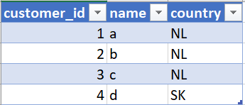
And another with sales data per customer called “SalesData:
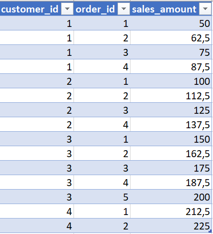
In the Customer table, we want to add to total sales amount per customer. We can use a subquery for this:

SELECT Customer.customer_id,
TotalSales.TotalAmount
FROM Customer
INNER JOIN
(SELECT customer_id,
SUM(sales_amount) as TotalAmount
FROM
SalesData
GROUP BY customer_id) as TotalSales
on customer.customer_ID = TotalSales.customer_ID

In the example above, we use the subquery to select the total sales per customer which we then join to our customer data.

CTE (Common Table Expression)

A CTE is, just like a subquery, a result of a select statement that is defined in the query itself. In most cases, a CTE can serve the same purpose as a subquery. A CTE always starts with the “WITH” clause, after which the CTE’s select statement is written. Let’s create a CTE to get exactly the same result as the sub query above:

WITH TotalSales AS
(SELECT customer_id,
SUM(sales.sales_amount) as TotalAmount
FROM Sales
GROUP BY customer_id)

SELECT customer.customer_id,
TotalSales.TotalAmount
FROM customer
INNER JOIN TotalSales
on customer.customer_id = TotalSales.customer_id

In the example above, we first create a CTE which generates the total sales amount per customer. In the SELECT statement that follows, we join in the CTE we just created to get the total sales amount per customer. When we need to use multiple CTE’s in one query, we always start with writing all the CTE’s in the beginning of the query and then referring to them afterwards, like so:

WITH CTE1 as (SELECT * FROM TABLE1),
CTE2 as (SELECT * FROM TABLE2),
CTE3 as (SELECT * FROM TABLE3),
CTE4 as (SELECT * FROM TABLE4)

SELECT * FROM CTE1
UNION
SELECT * FROM CTE2
UNION
SELECT * FROM CTE3
UNION 
SELECT * FROM CTE4

This standard structure of the query, makes it more readable. However, opinions about readability of CTE’s vary as people are used to their own way of writing SQL queries.

(Functional) differences between sub queries and CTE’s

  • Subqueries can be defined anywhere in the query. CTE’s have to be declared in the beginning of the query after which they can be referred to
  • Subqueries can be used with WHERE clause in combination with IN and EXISTS keywords to filter the data. CTE’s do not allow you to do this. An example of this will be shared below
  • CTE’s enable recursive functionality. An example of this will be shared below.
  • CTE’s are defined in the beginning of the query, and subqueries are defined inline
  • CTE’s always have to be defined with a name (this is not required for subqueries, but it is best practice to do so)
  • CTE’s can be referred to multiple times in the SQL query, subqueries can only be used once
  • Subqueries can be used to update the contents of the table, CTE’s do not offer this functionality

Subquery exclusive: using IN keyword

We have two tables with employee data. The first table, called EMPMASTER, contains some employee master data:

The second table, called EMPSCALE, contains data related to the payscales of employees:

If we want to filter the first table based on the contents of the second table, without joining, we can use the following code in which we use the WHERE clause in combination with the IN keyword that is using a subquery as the source:

SELECT * FROM EMPMASTER
WHERE EmpNumber IN(
  SELECT EmpNumber FROM EMPSCALE WHERE Payscale >13)

This particular example cannot be recreated by using a CTE.

CTE exclusive: recursive queries

A big strength of a CTE is the ability to be recursive. Recursive queries makes it possible to work with hierarchical data. This can be rather useful when looking at the hierarchy in an organization in which every manager has a manager until we reach the CEO. With the recursive CTE, we can indicate the hierarchy levels of the employees within a organization. A full explanation of recursive CTE’s and its use will be shared in a future blogpost.

Conclusion

In this blogpost we have touched upon the functional difference between a CTE and a subquery. Based on those differences, we can make a decision to choose one of the two options. Generally speaking, people tend to find that CTE’s make the query more readable, but this is mostly based on personal preference. The general misconception that CTE’s are are more efficient that subqueries because the data is temporarily stored, is false. If performance is an important aspect, it is better to create a temp table with an index, which both the CTE and subquery cannot offer.

Reproducing the SQL LAG function in Power Query in order to determine an internal promotion

People that start using Power Query after getting experience in SQL tend to miss the wide range of options that SQL gives. Power Query actually has lots of powerful options available and most of the use cases can be solved by only using the UI.

In this blog I will explain how to recreate the SQL lag function in power query by using only the UI. In order to understand this, we first have to get familiar with the SQL lag function as well as Common Table Expressions (CTE).

The SQL way

Let’s say that we have an employee details table called employee_data, which has the following columns:

Employee_number

Change_event

Cost_center

Payscale

Start_date

End_date

Let’s create this table in SQL:

CREATE TABLE employee_data (
employee_number serial,
change_event VARCHAR ( 30) NOT NULL,
cost_center varchar (4) NOT NULL, 
payscale VARCHAR (1) NOT NULL,
start_date DATE NOT NULL,
end_date DATE NOT NULL
)

After inserting some dummy data, the contents of the table look like this:

This is data from an event-based ERP. Based on the events, new records are created with new start and end dates. In order to determine if someone has been promoted, we have to compare the current row against the previous row. To make it simple; if the previous row’s payscale was A and the current row’s payscale is B, the employee had a payscale increase (B is an higher payscale than A).

In the current dataset, there is one internal promotion happening for employee 1 as he goes from A to B on 01-06-2020:

To get the previous row, we will need the SQL lag function. However, as the SQL lag function requires it to be included in a window function we need additional logic. (the SQL Window function and all its details will be discussed in detail in a future blogpost). The following code will retrieve the previous row for the payscale column:

LAG(payscale,1)
OVER ()
FROM EMPLOYEE_DATA

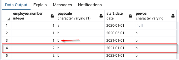
The challenge is that it will always retrieve the previous row. In our use case we only need the previous row for the same employee. If we always get the previous row, we will end up mixing data from multiple employees:

In screenshot above, you can see that the prevps column is displaying the value ‘b’ for employee 2, and the ‘b’ value is actually the value that belongs to employee 1.

In order to get the previous row per employee we will need to use the PARTITION BY part:

SELECT employee_number, 
payscale, 
start_date,
LAG(payscale,1)
OVER (PARTITION BY employee_number ORDER BY start_date) as prevps
FROM EMPLOYEE_DATA
ORDER by employee_number, start_date

This will result in the following output in which there will be a ‘null’ value for the cases that there is no previous row for the concerned employee:

We can now compare the previous row’s payscale against the current row’s payscale in order to determine if there was a promotion. However, SQL does not allow the newly created column (prevps), to be used in the same SELECT statement. In order to tackle this, we will use the above SELECT statement in a Common Table Expression (CTE):

WITH promotion_table AS
(SELECT employee_number, 
payscale, 
start_date,
LAG(payscale,1)
OVER (PARTITION BY employee_number ORDER BY start_date) as prevps
FROM EMPLOYEE_DATA
ORDER by employee_number, start_date)

SELECT * FROM promotion_table
WHERE payscale > prevps

What this does is:

  • It first creates a temporary table via the CTE
  • We can then query this temporary table by our 2nd select statement
  • In the 2nd select statement we indicate we only want to see the records where the current payscale is higher than the previous payscale (prevps). Fun fact: you can actually compare textual values in a logical way in SQL, e.g.: B > A = TRUE

The Power Query way

We have exactly the same data in our Power Query dataset, and all data types are correctly indicated:

Power Query does not offer standard functionality to retrieve the previous row. We can however still accomplish this by applying a self-join. Before applying this logic, it is important to first sort the rows correctly. We want to sort the rows ascending based on employee_number and start_date:

Table.Sort(#"Changed Type",{{"employee_number", Order.Ascending}, {"start_date", Order.Ascending}})

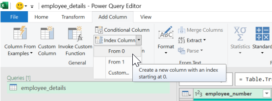
After sorting the rows correctly, we can proceed with adding 2 separate index columns via add column ribbon -> Index Column:

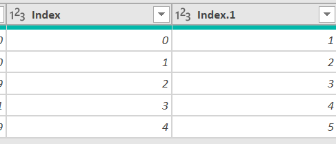
An index column is nothing more than a column that increments by a certain value. We need one index column to start counting from 0 and another starting from 1. After applying this, our 2 new columns should be visible:

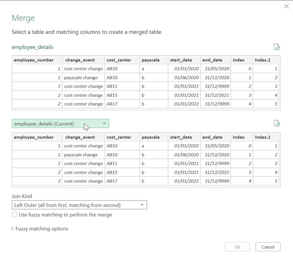
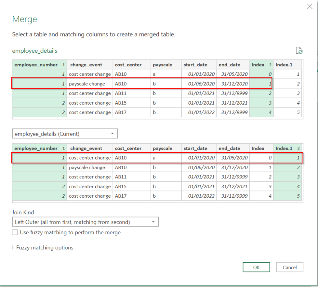
Now we have added the two index columns, we can proceed with applying the self join. In the Home ribbon we click on Merge Queries. In the window that pops up we select our employee_details table:

This is the basis for our self-join. The next step is to determine the elements of our self join. For this we select the employee_number column and the two separate index columns:

So now we have joined our table on itself, but based on different elements. For each employee number, we want to retrieve the previous row. In the example above, the elements of the main query are employee 1 and index 1. The join is going to search for those elements in the second query (which is still our main table), and it’s going to search for the combination of employee 1 and index 1. Since we have selected the different index column in our joined query, it is going to find this combination in the previous row (see the second red outlined element in example above).

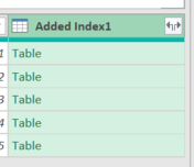
After applying the self-join, Power Query will create this nested table in which the tables are stored that contain the previous row values:

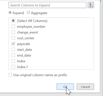
We can expand this nested table, and select the desired columns. We are only interested in the payscale column as we want to compare the current payscale against the previous payscale. Let’s expand this column:

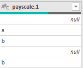
Power Query will give the new column that is added, the ‘.1’ trailing text via this automatically generated code:

= Table.ExpandTableColumn(#"Merged Queries", "Added Index1", {"payscale"}, {"payscale.1"})

We can change this new column name without creating a new step by changing the created step to:

= Table.ExpandTableColumn(#"Merged Queries", "Added Index1", {"payscale"}, {"prevps"})

This results in the following dataset:

Based on this data we can determine the internal promotions by comparing the current row’s payscale against the previous row’s payscale. Let’s create the required logic in a custom column. In the Add Column ribbon, click on Custom Column. In the window that pops up, we give our new column a new name and add the following logic:

if [prevps] = null then "no promotion" else if [payscale] > [prevps] then "promotion" else "no promotion"

This will result in the following final column in which the promotion is indicated:

The fact that we can accomplish the required output using solely the UI in Power Query is a powerful thing. We do need to take into account the impact joins have on the performance of the query, which will be covered in a future blogpost.