Everything BI

Excel, Power Query M code, SQL,

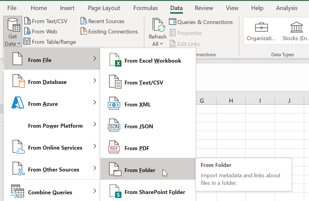
Using custom functions in Power Query (to boost performance)

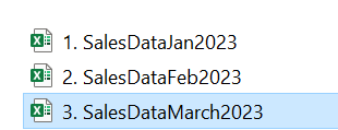
In this blogpost we have seen how to import multiple Excel files from a folder. During this process, we have imported all sales data from the various sales representatives and afterwards expanded all of the nested tables, which in return combined all of the data. In this particular example, the combined Excel files resulted in 150.000 rows total, which is still easily handled by Power Query. But let’s imagine an example in which we import 10 files with 100.000 rows each. After combining the Excel files, the total amount of rows will be 1 million. If all data is relevant, this should not be an issue. But what if we only need the data for one of the many sales representatives, which is only 25.000 rows total? If we combine all of the data, Power Query will expand the nested tables to 1 million rows and we can filter on the relevant sales representative afterwards, but the fact that we are expanding all 1 million rows will have a negative impact on the performance. What if there was a way to filter all of the nested tables before expanding the data? That’s were a custom function can come in handy. In order to understand how to write a custom function, we first need some basic knowledge of the M-code that Power Query generates when applying query steps.

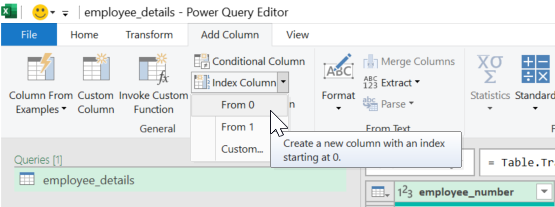
The Power Query M-language

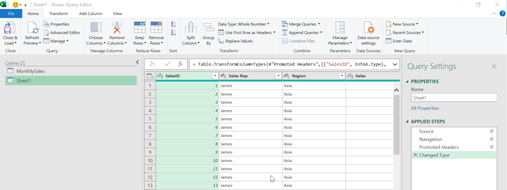
When using the user interface, Power Query will generate multiple query steps for you:

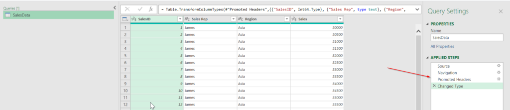
In the screenshot above we have applied the following steps:

  1. Source: import Excel file
  2. Navigation: navigate to relevant object in the Excel file
  3. Promoted Headers: used the first row as headers
  4. Changed Type: changed the datatype of all of the columns

All of those steps that we apply via the user interface, generate M-code on the background. If we now click on the advanced editor, we can see the M-code that was generated:

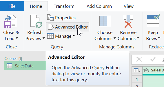
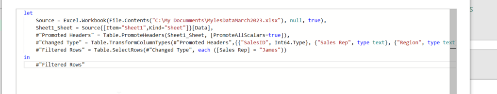
In the advanced editor we can see the following code:

In the code above, we can find our query steps. The way Power Query works, is that it first defines all of the expression steps (query steps) after the “let” expression. After the “let” expression, all expression steps are composed and form the mashup query. in the final step, the last expression step is outputted after the “in” expression. Each of the expression steps start with the query step name, for example #”Changed Type” after which the relevant M-code is written. In the example above, each step starts with a function, such as “Table.TransformColumnTypes”. The first parameter of a function is always the name of the previous step. If we look at the #”Changed Type” step, the Table.TransformColumnTypes function takes the “Promoted Headers” step as the first parameter, which is the previous query step. This little piece of basic information will help us understand how to build our custom function. A future blogpost will be dedicated to the Power Query M-language and the way the engine works.

Building the custom function

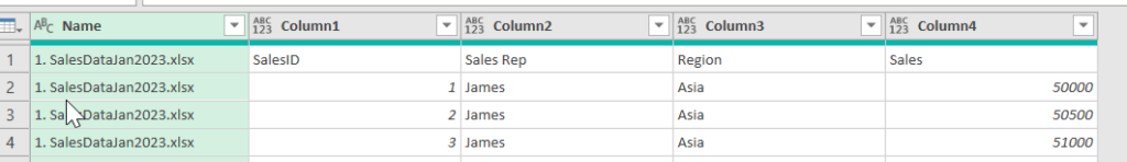
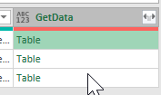
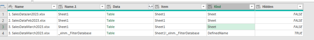
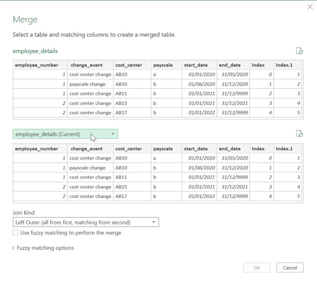
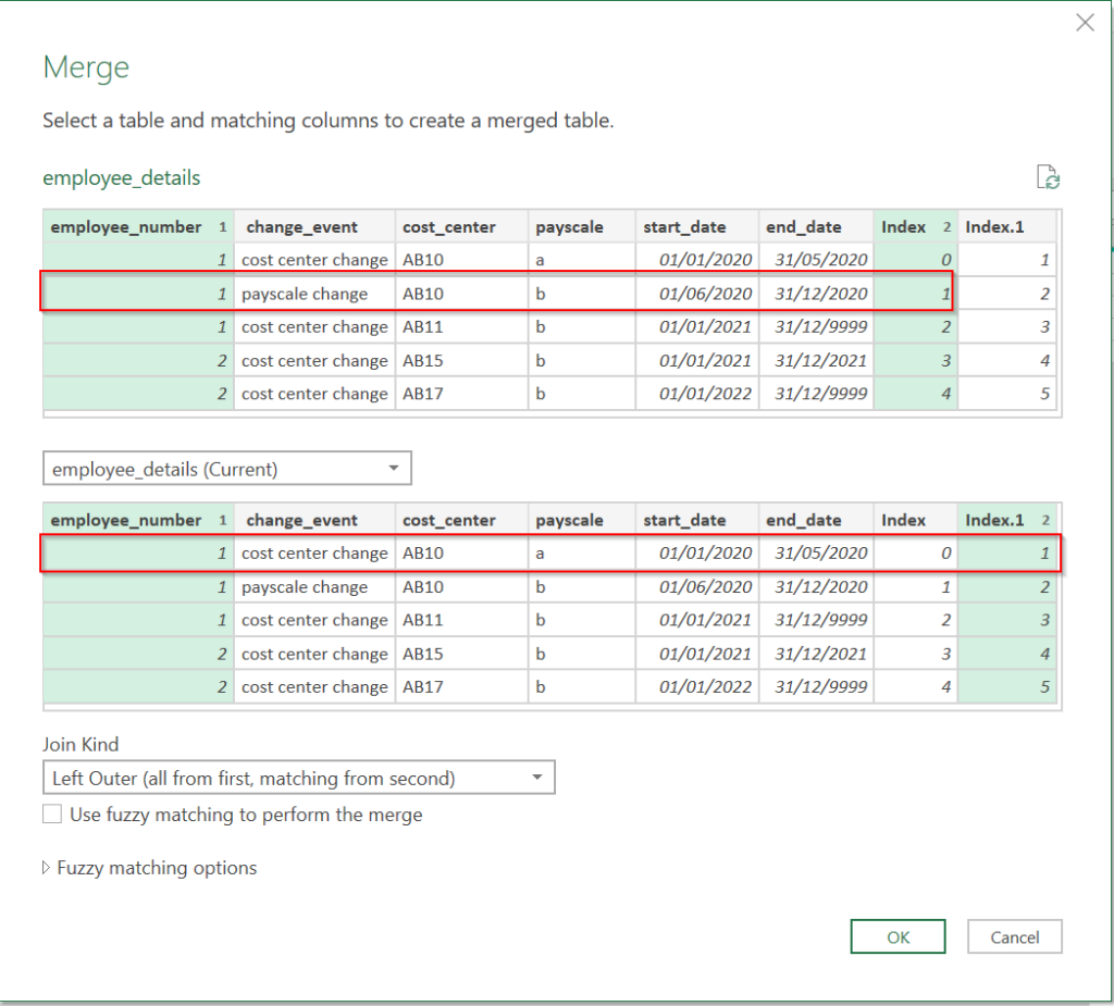
In the earlier blogpost, we expanded all the data and then applied our data manipulation steps afterwards. This means that when looking at the situation in the screenshot below, we would expand all the data that is stored in the nested tables in the 2nd column:

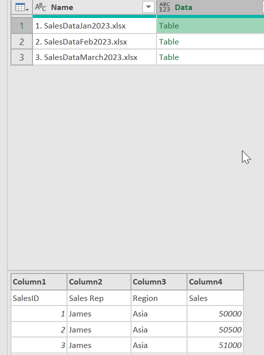
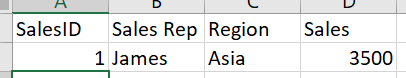
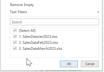
If we need all the data, that is perfectly fine. But let’s imagine that we only need the data for the sales representative James. In this case it would be efficient to filter the nested tables to only contain data for sales representative James and expanding the nested tables afterwards. Nested tables can be manipulated just like a regular table (as we are doing when using the User Interface), but we need to apply all of the query steps in the nested table itself. Now we first need to determine what data manipulation steps we want to apply to the nested tables. For this we import one single sales file to Power Query (it does not matter which file, any of the files in the folder is fine):

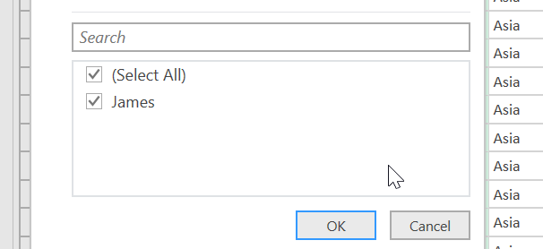
We are not going to actually use this query, we are just getting the relevant code from it. The “Promoted Headers” and the “Changed Type” steps are automatically generated by Power Query. The next thing we want to do, is filter the data to only include data for James:

After applying this filter, a new “Filtered Rows” step is added:

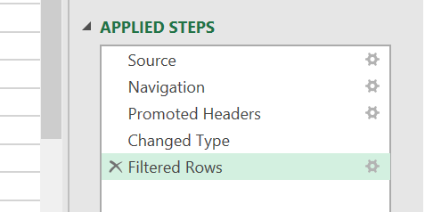
The steps that we now have applied, are the steps that we want to apply to all the nested tables:

  • First we want to promote the headers
  • Then we want to change the datatype of the columns
  • Finally we want to filter the table to only contain data for James

Let’s have a quick look at the M-code that has been generated via the three query steps:

#"Promoted Headers" = Table.PromoteHeaders(Sheet1_Sheet, [PromoteAllScalars=true]),
    #"Changed Type" = Table.TransformColumnTypes(#"Promoted Headers",{{"SalesID", Int64.Type}, {"Sales Rep", type text}, {"Region", type text}, {"Sales", Int64.Type}}),
    #"Filtered Rows" = Table.SelectRows(#"Changed Type", each ([Sales Rep] = "James"))

We can find the all of the three steps in the code above. Those three query steps is what we want to apply to our nested tables. If we go back to the advanced editor to see the full M-code, we can find additional query steps:

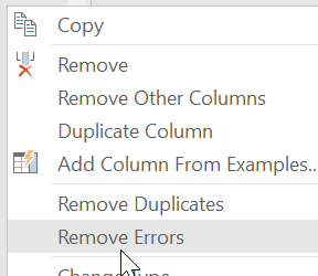
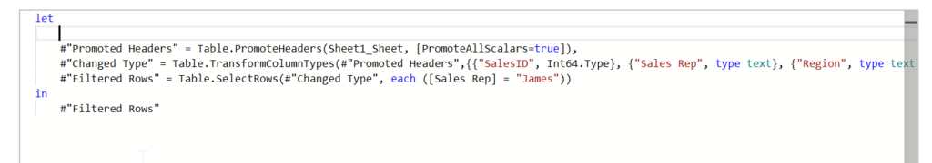
The source step and the navigation step (the first 2 steps) are not relevant for us. This because we already have defined the source and the navigation steps in our main query, which resulted in the nested tables. We are only interested in the “Promoted Headers”, “Changed Type”, and “Filtered Rows” steps. We will remove the first two steps:

The next step is to transform the M-code above into a custom function. We can use the following operator to start a custom function:
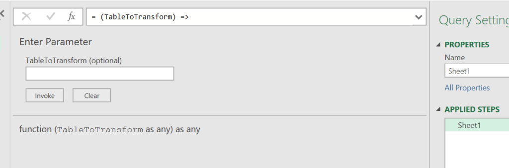
=>

Before the custom function operator, we have to specify our input parameters and afterwards the relevant M-code will follow. Let’s start our custom function:

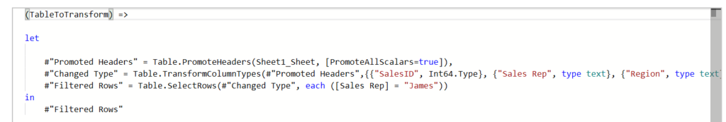
In the example above, our input parameter is called “TableToTransform” which is followed by the relevant M-code containing the query steps that we want to apply. Since each applied query step will always start with a reference to the previous query step, the code above is not yet complete.

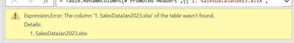
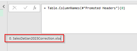
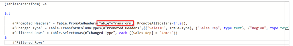
The first query step still refers to the previous step in the old situation. We have stripped this M-code down, so this will not work. The first query step has to be applied to our nested table. In the custom function we are passing the nested tables as input parameters, and since we have created our TableToTransform input parameter, we can use this in the first query step:

If we click done, our custom function has been built:

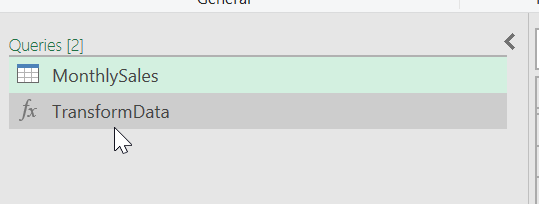
In our Queries overview, we can now also find the custom function, which has been renamed to TransformData:

When we will use the custom function, it will do the following:

  1. It will take the nested table as the input
  2. In the nested table, the first rows will be promoted as headers
  3. In the nested table, the datatypes will be changed
  4. In the nested table, a filter will be applied to only include sales data for James

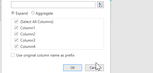
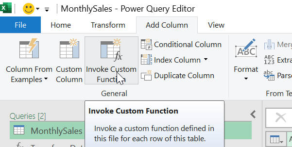
Now let’s use our created custom function. For this we go back to our query with the nested tables and click on “Invoke Custom Function”:

The following windows pops up:

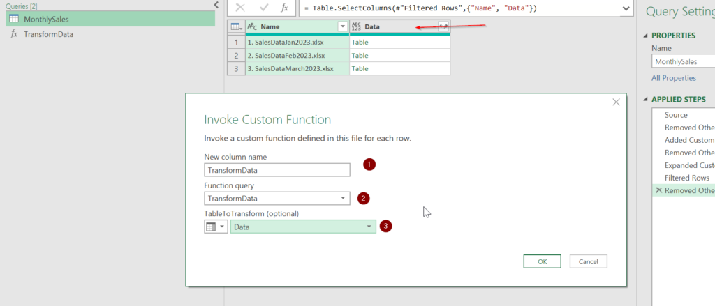
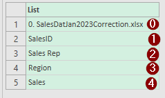
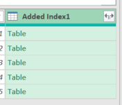
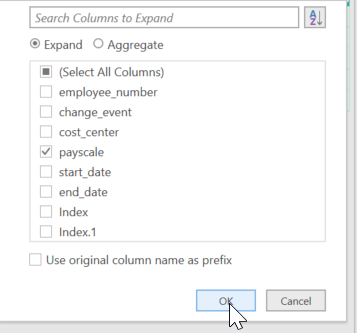
In the first window, we specify the new column name. In the second window we choose the function the we want to use, TransformData in this case (we only have one available function). In the third window we have to specify which column we want to use the function on. Since the “Data” column holds all of our nested tables, we choose this column. After clicking on “OK” the function is applied and a new column appears:

This new column again, holds nested tables, but those tables contain data that has been manipulated based on our function:

  • The first row is promoted to headers
  • The datatypes are changed
  • The table only contains data for James

Now let’s remove the column with the old nested tables:

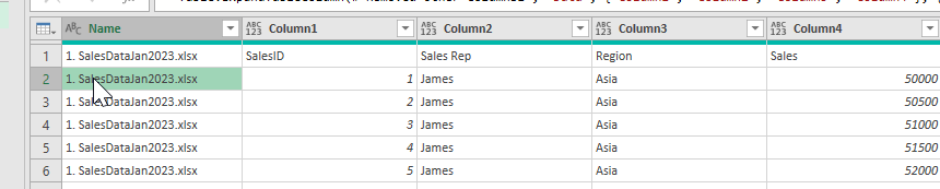
After expanding our new nested tables, only data for James is expanded:

In this rather simple example, we can see the power of a custom function. Custom functions can be used in a wide range of situations to increase efficiency but also to help with complex transformations. In a future blogpost I will demonstrate how a custom function can be used to tackle a complex transformation challenge. Only when you are aware of the power of custom functions, you will start to see use cases during your own work…

Dynamically renaming columns in Power Query

The fact that a rename columns step in Power Query is hard-coded, has resulted in some challenges for many people. Of course, when we import data, the names of the columns and the structure should always remain the same in the source. If this isn’t the case, our steps in which the columns names are hard-coded, will result in errors and this is an expected result. However, if we look at this blogpost in which we imported files from a folder, we still have this challenge even though the structure of our source files do not change.

Let’s pick up where we left last time. After importing the files, our data looks like this:

Now we have to promote the first row as headers in order to get the correct column names:

Now all columns have a correct column name, but the first column does not. Because the filename is linked to all of the rows in the three files, the filename will be promoted as a header. In this case the column name is not correct as we want to call this column “ConcernedFile”. Let’s rename the column:

= Table.RenameColumns(#"Promoted Headers",{{"1. SalesDataJan2023.xlsx", "ConcernedFile"}})

As you can see in the code above, the column name that we want to rename (“1. SalesDataJan2023.xlsx”) is hard-coded. This means that if in a future situation, when the files in the folder are sorted in a different way, or when new files are added, the first file could be a different one. What then happens is that Power Query tries to rename the column based on the hard-coded column name, even though the column now has a different name e.g. “0. SalesDatJan2023Correction.xlsx”. This will result in an error and the query will break:

In this case, we do not want to rename the first column based on its name but based on its position. This because we know that the first column will always be the filename one. In this example we have 5 columns and we always want to rename the first column to “ConcernedFile”. Before we proceed with customizing our M code to accomplish this, we first have to understand what the Renamed Columns step is doing syntax-wise:

= Table.RenameColumns(#"Promoted Headers",{{"0. SalesDatJan2023Correction.xlsx", "ConcernedFile"}, {"SalesID", "SalesTest"}})

In the code above, we are renaming the 0. SalesDatJan2023Correction.xlsx column to ConcernedFile and we rename SalesID to SalesTest.

The first part before the comma is always a reference to the previous step in the query, in this case #”Promoted Headers”. In the next part, Power Query requires a list of column pairs that we want to rename. In the following column pair that is wrapped in a list, we specify that we want to rename “0. SalesDatJan2023Correction.xlsx” to “ConcernedFile”:

{"0. SalesDatJan2023Correction.xlsx", "ConcernedYear"}

The fact that those columns are wrapped in {}, makes it a list. Power Query requires all of those column pairs in separate lists that is wrapped in another list:

{{"0. SalesDatJan2023Correction.xlsx", "ConcernedYear"}, {"SalesID", "SalesTest"}}

Now that we have a better understanding of the syntax of the renamed columns step, we can start modifying the code to make it dynamic. For this, we also need the Table.ColumnNames function. This function simply creates a list of all columns in the table. The only parameter is the name of the previous step, so if we apply this function in our query:

Table.ColumnNames(#"Promoted Headers")

We will get the following list of column names:

The first column is the one that we want to rename to ConcernedFile. Based on the list above, we can retrieve single values by specifying which column we want to see based on its order (index) in the list. Power Query starts counting from 0, so number 0 is the column we want to rename. In order to retrieve single values from a list, we can use the positional index operator, which requires the number to again be wrapped in curly brackets {}. The following code will retrieve the first (0st) value from the list above:

= Table.ColumnNames(#"Promoted Headers"){0}

It will result in a singe value:

The single value that we have retrieved with the code above, can be used in our Renamed Columns step. Our initial code was:

= Table.RenameColumns(#"Promoted Headers",{{"0. SalesDatJan2023Correction.xlsx", "ConcernedFile"}, {"SalesID", "SalesTest"}})

We want to make the “0. SalesDatJan2023Correction.xlsx” part dynamic, so we adjust the code to:

= Table.RenameColumns(#"Promoted Headers",{{Table.ColumnNames(#"Promoted Headers"){0}, "ConcernedFile"}, {"SalesID", "SalesTest"}})

And that’s it. Now every time the query is refreshed, the first column will dynamically be renamed. The other columns, which are hard-coded, are fine because we know that the structure of our sources should not and will not change.

Importing files from a folder using Power Query

Power Query offers lots of options when it comes to importing data. Importing files from a folder is one of them, and it can result in significant time saving as multiple files can all be transformed based on the applied query steps. Let’s have a look at one practical example.

Our fictive company saves monthly sales reports, in a specific shared folder. All data is saved as separate .xlsx files for the concerned month. The month name and the year are always included in the filename. We currently only have data available for the first 3 months of 2023:

All of the reports contain the following 3 columns:

Column A displays the sales ID, column B displays the name of the sales representative (either James or Olivier), column C displays the region (either Asia or Europe), and column D displays the sales amount in EUR. Every first day of the month, after a new sales report is added to the folder, some colleague is manually copy pasting the data into a Masterfile and updating their formulas. This is a risky and inefficient process and Power Query offers the solution.

Importing the data from a folder

First we start by selecting from folder in the get data section in Power Query and paste the folder path:

Power Query then automatically generates the following columns based on the folder path and file details:

The first column Content contains the contents of the separate Excel file. Column B displays the file name and the rest of the columns are specific details of the separate Excel files. In order to read the data, we have create a custom column and use the following function:

Excel.Workbook([Content])

This particular function reads all of the objects from the separate Excel files and it will generate this new column:

The new column contains nested tables with all of the objects from the Excel files. We can expand the contents and Power Query will show all of the objects that it has read from the Excel files. 5 new columns are generated:

The column Item displays the items that it could read from the Excel files and column Kind displays what time of item it concerns. Power Query is able to read Tables, named ranges, dynamic arrays and sheets. In this example we know that the data that we are interested in, is always located in a sheet named Sheet1. To make sure that Power Query always imports the correct data, we apply a filter on the Item column and filter only on Sheet1 values:

After applying the filter, we are left with only relevant records. Now that we have applied our filtering, we can delete all columns besides Name and Data. The Name column contains the name of the file which we can use to determine the sales month and year. The column Data that was created by Power Query contains nested tables with the actual contents that we are interested in. Now we can proceed with expanding the data:

After expanding, we have all the data, of all three Excel files combined:

Now we can promote the first row as headers and validate that all data is included by checking the available values in column A:

Based on information above, we can confirm that we have successfully combined all the data from the three separate Excel files. However, as Power Query combines all data in the Excel files, it also combines the header data. That means that the Sales column does not only contain the sales value, but actually also contains 2 “Sales” values. As the Sales column has a numeric datatype combined with the fact that Power Query is datatype sensitive, there will errors in the dataset. We can fix this by applying a Remove Errors step on the Sales column:

This step will remove all the errors based on the datatype of the Sales column, so it will remove all records that are not a numeric datatype. The data can now be used and analyzed. If there will be new files added to the folder that we have linked our Power Query to, they will be automatically included once the query is refreshed. This means that the transformation will automatically by applied to all files in the folder based on our query steps.

Reproducing the SQL LAG function in Power Query in order to determine an internal promotion

People that start using Power Query after getting experience in SQL tend to miss the wide range of options that SQL gives. Power Query actually has lots of powerful options available and most of the use cases can be solved by only using the UI.

In this blog I will explain how to recreate the SQL lag function in power query by using only the UI. In order to understand this, we first have to get familiar with the SQL lag function as well as Common Table Expressions (CTE).

The SQL way

Let’s say that we have an employee details table called employee_data, which has the following columns:

Employee_number

Change_event

Cost_center

Payscale

Start_date

End_date

Let’s create this table in SQL:

CREATE TABLE employee_data (
employee_number serial,
change_event VARCHAR ( 30) NOT NULL,
cost_center varchar (4) NOT NULL, 
payscale VARCHAR (1) NOT NULL,
start_date DATE NOT NULL,
end_date DATE NOT NULL
)

After inserting some dummy data, the contents of the table look like this:

This is data from an event-based ERP. Based on the events, new records are created with new start and end dates. In order to determine if someone has been promoted, we have to compare the current row against the previous row. To make it simple; if the previous row’s payscale was A and the current row’s payscale is B, the employee had a payscale increase (B is an higher payscale than A).

In the current dataset, there is one internal promotion happening for employee 1 as he goes from A to B on 01-06-2020:

To get the previous row, we will need the SQL lag function. However, as the SQL lag function requires it to be included in a window function we need additional logic. (the SQL Window function and all its details will be discussed in detail in a future blogpost). The following code will retrieve the previous row for the payscale column:

LAG(payscale,1)
OVER ()
FROM EMPLOYEE_DATA

The challenge is that it will always retrieve the previous row. In our use case we only need the previous row for the same employee. If we always get the previous row, we will end up mixing data from multiple employees:

In screenshot above, you can see that the prevps column is displaying the value ‘b’ for employee 2, and the ‘b’ value is actually the value that belongs to employee 1.

In order to get the previous row per employee we will need to use the PARTITION BY part:

SELECT employee_number, 
payscale, 
start_date,
LAG(payscale,1)
OVER (PARTITION BY employee_number ORDER BY start_date) as prevps
FROM EMPLOYEE_DATA
ORDER by employee_number, start_date

This will result in the following output in which there will be a ‘null’ value for the cases that there is no previous row for the concerned employee:

We can now compare the previous row’s payscale against the current row’s payscale in order to determine if there was a promotion. However, SQL does not allow the newly created column (prevps), to be used in the same SELECT statement. In order to tackle this, we will use the above SELECT statement in a Common Table Expression (CTE):

WITH promotion_table AS
(SELECT employee_number, 
payscale, 
start_date,
LAG(payscale,1)
OVER (PARTITION BY employee_number ORDER BY start_date) as prevps
FROM EMPLOYEE_DATA
ORDER by employee_number, start_date)

SELECT * FROM promotion_table
WHERE payscale > prevps

What this does is:

  • It first creates a temporary table via the CTE
  • We can then query this temporary table by our 2nd select statement
  • In the 2nd select statement we indicate we only want to see the records where the current payscale is higher than the previous payscale (prevps). Fun fact: you can actually compare textual values in a logical way in SQL, e.g.: B > A = TRUE

The Power Query way

We have exactly the same data in our Power Query dataset, and all data types are correctly indicated:

Power Query does not offer standard functionality to retrieve the previous row. We can however still accomplish this by applying a self-join. Before applying this logic, it is important to first sort the rows correctly. We want to sort the rows ascending based on employee_number and start_date:

Table.Sort(#"Changed Type",{{"employee_number", Order.Ascending}, {"start_date", Order.Ascending}})

After sorting the rows correctly, we can proceed with adding 2 separate index columns via add column ribbon -> Index Column:

An index column is nothing more than a column that increments by a certain value. We need one index column to start counting from 0 and another starting from 1. After applying this, our 2 new columns should be visible:

Now we have added the two index columns, we can proceed with applying the self join. In the Home ribbon we click on Merge Queries. In the window that pops up we select our employee_details table:

This is the basis for our self-join. The next step is to determine the elements of our self join. For this we select the employee_number column and the two separate index columns:

So now we have joined our table on itself, but based on different elements. For each employee number, we want to retrieve the previous row. In the example above, the elements of the main query are employee 1 and index 1. The join is going to search for those elements in the second query (which is still our main table), and it’s going to search for the combination of employee 1 and index 1. Since we have selected the different index column in our joined query, it is going to find this combination in the previous row (see the second red outlined element in example above).

After applying the self-join, Power Query will create this nested table in which the tables are stored that contain the previous row values:

We can expand this nested table, and select the desired columns. We are only interested in the payscale column as we want to compare the current payscale against the previous payscale. Let’s expand this column:

Power Query will give the new column that is added, the ‘.1’ trailing text via this automatically generated code:

= Table.ExpandTableColumn(#"Merged Queries", "Added Index1", {"payscale"}, {"payscale.1"})

We can change this new column name without creating a new step by changing the created step to:

= Table.ExpandTableColumn(#"Merged Queries", "Added Index1", {"payscale"}, {"prevps"})

This results in the following dataset:

Based on this data we can determine the internal promotions by comparing the current row’s payscale against the previous row’s payscale. Let’s create the required logic in a custom column. In the Add Column ribbon, click on Custom Column. In the window that pops up, we give our new column a new name and add the following logic:

if [prevps] = null then "no promotion" else if [payscale] > [prevps] then "promotion" else "no promotion"

This will result in the following final column in which the promotion is indicated:

The fact that we can accomplish the required output using solely the UI in Power Query is a powerful thing. We do need to take into account the impact joins have on the performance of the query, which will be covered in a future blogpost.